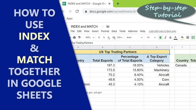
Google Sheets is a powerful tool for data analysis, and one of its most valuable functions is the combination of index match google sheets and MATCH. This duo offers a flexible alternative to the traditional VLOOKUP function, allowing users to perform lookups across rows and columns with ease. In this article, we’ll explore how to effectively use INDEX and MATCH in Google Sheets, complete with examples and tips to optimize your spreadsheet skills.

Understanding the Functions

INDEX and MATCH are two separate functions that, when combined, can perform complex lookups:

• INDEX(array, row_num, [column_num]): Returns the value of a cell in a specified row and column from a given range.
  • array: The range of cells to search.
  • row_num: The row number in the array from which to retrieve a value.
  • column_num: (optional) The column number from which to retrieve a value.
• MATCH(search_key, range, [match_type]): Searches for a specified value in a range and returns the relative position of that item.
  • search_key: The value you want to find.
  • range: The range of cells to search within.
  • match_type: (optional) Defines the type of match:
    • 1 for less than (array must be sorted in ascending order)
    • 0 for exact match
    • -1 for greater than (array must be sorted in descending order)

Combining INDEX and MATCH

The power of combining INDEX and MATCH lies in their ability to perform lookups in any direction—unlike VLOOKUP, which only searches left to right.

Syntax

The general syntax for combining these functions looks like this:

Example Scenario

Let’s say you have a simple dataset:

A	B	C
Name	Age	City
John	25	New York
Jane	30	Los Angeles
Mike	22	Chicago

Goal

You want to find the age of "Jane."

Using INDEX-MATCH

Here’s how to set up your formula:

1. Set up the formula in a cell where you want the result. For instance, in cell E1, type:

• Explanation:
  • MATCH("Jane", A2
    , 0) looks for "Jane" in the range A2
    and returns the row number (2 in this case).
  • INDEX(B2
    , 2) then retrieves the value from the second position of the range B2
    , which corresponds to Jane's age (30).

Benefits of Using INDEX-MATCH

1. Versatility: INDEX-MATCH can look up values in any direction, not limited to left-to-right.
2. Efficiency: It often performs better than VLOOKUP with large datasets.
3. No need for sorted data: Unlike MATCH with a match_type of 1 or -1, INDEX-MATCH does not require the data to be sorted.

Tips for Effective Use

• Error Handling: Wrap your formula in IFERROR to manage errors gracefully. For instance:

• Dynamic References: Use cell references instead of hardcoded values for more dynamic formulas. For example:

This allows you to input different names in cell E2 and retrieve corresponding ages easily.

Conclusion

The combination of INDEX and MATCH in Google Sheets is a powerful tool for data analysis and management. By mastering these functions, you can streamline your data retrieval processes, enhance your spreadsheet skills, and make more informed decisions based on accurate data insights. Whether you’re handling simple datasets or more complex spreadsheets, INDEX-MATCH is a game changer worth mastering. Happy spreadsheeting!